何为反差分解?
关于方差分解的数学原理,在 GUSTA ME 这篇文章 Variation partitioning 有非常清晰且容易理解的介绍。
引用经管之家网友 lovecather668 在var中方差分解的意义 中的回答:
VAR中的方差分解是分析影响内生变量的结构冲击的贡献度。例如,有好多行业产品的需求变动会对钢铁行业产品的需求变动产生影响,像建材行业、汽车行业、机械行业、家电行业。那么如果我们想要知道这4个行业的需求变化对钢铁行业的需求变化产生的影响哪个大、哪个小呢,就可以用方差分解来做。做出来的结果是用贡献率(百分比)来表示的,如假设结果是以上4个行业在某个时点上的贡献率分别为10%,12%,16%,20%(随时间的变化,这个贡献率也是在变化的),其意思是在该时点钢铁行业需求的变动,10%是建材行业的需求变动引起的,12%是汽车行业的需求变动引起的,以此类推…..
在生命科学的实际应用中,可以基于 RDA 结果得出不同类型的环境因素(如何气候、土壤性质以及植物)对生物群落组成(如土壤线虫群落、微生物群落)的解释程度。
Singh et al.(2018) 在 Scientific Report 上发表的文章《tropical forest conversion to rubber plantation affects soil micro- & mesofaunal community & diversity》中提到了一套完整的基于 RDA 的方差分解操作:
We performed a redundancy analysis (RDA) based variation partitioning analysis 57 to assess the relative effects of environmental and spatial variables on community composition. We used Hellinger transformed OTU abundance data as the response variable and two sets of explanatory variables which included environmental variables (pH, Ele, TOC, AP, GSW, SX, TN, and ST) and spatial variables (geographical co-ordinates for sampling sites), respectively. Before the RDA, the environmental variables with high variance inflation factor (VIF) >10 were eliminated to avoid collinearity among factors. The importance of environmental and spatial variables in explaining species composition was determined by an RDA analysis using Monte Carlo permutation tests (999 unrestricted permutations) followed by forward selection to remove the non-significant variables from each of the explanatory sets.
如何进行这样的方差分解流程(包括变量筛选以及变量集的显著性标注)就是今天这篇文章的重点。
使用 R 进行方差分解
正如大多数基于群落的分析方法相同,在 R 中进行方差分解同样离不开 vegan 包,主要依赖两个功能:
数据继续使用之前的文章《使用 ggplot2 可视化 RDA 结果》中使用的演示数据。
# suppressMessages will hide message from loading package, it makes the output clearer
library(tidyverse)
# col_types = cols() will suppress message about the column type to make the output clearer
df_com <- read_csv('../assets/2020-04-28-post/df_com_smp.csv', col_types = cols())
df_env <- read_csv('../assets/2020-04-28-post/df_env_smp.csv', col_types = cols())

# Take a glimpse about the structure of data frame
glimpse(df_com)
## Rows: 150
## Columns: 5
## $ pp <dbl> 2.5500000, 1.3110456, 8.2500000, 102.4900000, 21.3500000, 2.4900000…
## $ ba <dbl> 28.010000, 7.316707, 13.255000, 18.516667, 52.720000, 4.965000, 61.…
## $ fu <dbl> 2.5500000, 1.3378838, 3.3550000, 20.9466667, 14.8466667, 1.2450000,…
## $ pr <dbl> 2.5500000, 1.3378838, 0.0000000, 0.0000000, 0.0000000, 0.0000000, 4…
## $ om <dbl> 15.280000, 5.953381, 14.850000, 23.500000, 5.623333, 2.475000, 31.2…glimpse(df_env)## Rows: 150
## Columns: 13
## $ pH <dbl> -1.63965465, 0.94291257, -1.33875709, -1.20359469, -1.17624072, 0.…
## $ MOI <dbl> -0.1610384, -0.5549069, -0.2762522, -0.1658411, 1.0043821, 0.54673…
## $ TN <dbl> -0.116240631, -0.791972999, 0.199881689, -0.260084650, 0.291874957…
## $ TP <dbl> -0.44892589, 0.02952209, -0.14900328, -0.45606691, -0.47748995, -0…
## $ AP <dbl> 0.17966965, -0.78701735, -0.10273314, 0.09277663, 2.24338416, 0.54…
## $ NH4 <dbl> 0.4471754, -0.3426843, 0.7179844, -0.1328073, 0.7924569, -0.365251…
## $ NO3 <dbl> -0.51485153, -0.41977560, -0.49221441, -0.16774892, -0.58276291, -…
## $ SOC <dbl> -0.292278803, -0.697789311, 0.461059956, -0.007572046, 0.035809220…
## $ MAT <dbl> 0.84202205, -1.55196703, -0.84801694, 0.78335952, -0.28932636, -0.…
## $ MAP <dbl> 0.02487222, 0.27013035, 1.21243154, -0.87351309, -0.22471654, 1.21…
## $ PBM <dbl> 0.17638650, -0.02465146, 0.73829039, -0.80968336, 0.12645186, 2.11…
## $ PCV <dbl> 0.426595458, 0.008333099, -0.793336422, -0.514494850, 0.182609082,…
## $ PSR <dbl> 0.22757812, -0.83529465, 0.83493399, -1.29081156, 0.98677296, 0.68…按照 varpart 在文档中的说明:
The functions partition the variation in Y into components accounted for by two to four explanatory tables and their combined effects. If Y is a multicolumn data frame or matrix, the partitioning is based on redundancy analysis (RDA, see rda), and if Y is a single variable, the partitioning is based on linear regression. If Y are dissimilarities, the decomposition is based on distance-based redundancy analysis (db-RDA, see capscale) following McArdle & Anderson (2001). The input dissimilarities must be compatible to the results of dist. Vegan functions vegdist, designdist, raupcrick and betadiver produce such objects, as do many other dissimilarity functions in R packages. However, symmetric square matrices are not recognized as dissimilarities but must be transformed with as.dist. Partitioning will be made to squared dissimilarities analogously to using variance with rectangular data – unless sqrt.dist = TRUE was specified.
对于群落矩阵,方差分解是按照 RDA 结果来进行处理的,因此筛选变量的流程可在 RDA 分析的过程中完成。
为何要筛选变量?
在多因素的分析中,例如 RDA 分析和多元线性回归,任何增加新的变量,都会使得模型「看起来」拟合得更好,然而实际情况显然并非如此,为了解决过拟合问题调整 R 方是一个很常用的指标,具体的解释可以查看 Adjusted R2 / Adjusted R-Squared: What is it used for?。
回到正题,对于 RDA 分析选择变量,ordistep 提供了三种方法 backward, forward, both,即从全模型逐渐消除变量、从零模型逐渐增加变量以及双向选择变量。这里我们同时进行三种变量选择的方式。
# suppressMessages will hide message from loading package, it makes the output clearer
suppressMessages(library(vegan))

# Create the full model
rda_full <- rda(df_com~., data = df_env)

# Create the zero model
rda_null <- rda(df_com~1, data = df_env)

# backward selection
# trace = 0 prevent ordistep print the selection progress from outputing to the console
# it makes the output clearer.
rda_back <- ordistep(rda_full, direction = 'backward',trace = 0)

# forward selection
rda_frwd <- ordistep(rda_null, formula(rda_full), direction = 'forward',trace = 0)

# bothward selection
rda_both <- ordistep(rda_null, formula(rda_full), direction = 'both',trace = 0)

rda_back
## Call: rda(formula = df_com ~ pH + MOI + TN + TP + NO3 + SOC + MAT, data
## = df_env)
##
## Inertia Proportion Rank
## Total 2031.7341 1.0000
## Constrained 860.1782 0.4234 5
## Unconstrained 1171.5559 0.5766 5
## Inertia is variance
##
## Eigenvalues for constrained axes:
## RDA1 RDA2 RDA3 RDA4 RDA5
## 747.1 77.3 32.2 2.5 1.0
##
## Eigenvalues for unconstrained axes:
## PC1 PC2 PC3 PC4 PC5
## 755.6 247.3 108.6 46.6 13.5rda_frwd## Call: rda(formula = df_com ~ MOI + TN + SOC + NO3, data = df_env)
##
## Inertia Proportion Rank
## Total 2031.7341 1.0000
## Constrained 790.2092 0.3889 4
## Unconstrained 1241.5248 0.6111 5
## Inertia is variance
##
## Eigenvalues for constrained axes:
## RDA1 RDA2 RDA3 RDA4
## 714.8 70.1 4.3 1.0
##
## Eigenvalues for unconstrained axes:
## PC1 PC2 PC3 PC4 PC5
## 787.6 277.0 114.1 48.7 14.0rda_both## Call: rda(formula = df_com ~ MOI + NO3 + TN + SOC + TP + pH, data =
## df_env)
##
## Inertia Proportion Rank
## Total 2031.7341 1.0000
## Constrained 838.3620 0.4126 5
## Unconstrained 1193.3721 0.5874 5
## Inertia is variance
##
## Eigenvalues for constrained axes:
## RDA1 RDA2 RDA3 RDA4 RDA5
## 736.0 70.9 28.9 2.1 0.4
##
## Eigenvalues for unconstrained axes:
## PC1 PC2 PC3 PC4 PC5
## 769.5 253.1 110.3 46.6 13.9根据实际情况选择最终的模型,这里我们选择向后消除法选择的模型作为 RDA 最终的结果。同时这也是方差分解的最终模型,即 df_com ~ pH + MOI + TN + TP + NO3 + SOC + MAT,其中 MAT 是气候因素,我们将其选入气候因素集 df_clim, 其余均为土壤性质因素集 df_soil,植物因素没有选入模型。
# Divide the environmental data.frame by different categories.
df_clim <- df_env %>% select(MAT)
df_soil <- df_env %>% select(pH,MOI,TN,TP,NO3,SOC)

# Perform variation partitioning analysis, the first variable is the community matrix
# the second and third variables are climate variable set and soil property variable set
vpt <- varpart(df_com, df_clim, df_soil)

vpt

plot(
    vpt,
    bg = 2:5,
    id.size = 1.1,
    cex = 1.2,
    Xnames = c('Climate', 'Soil properties')
)
title('Variation partitioning by varpart from vegan')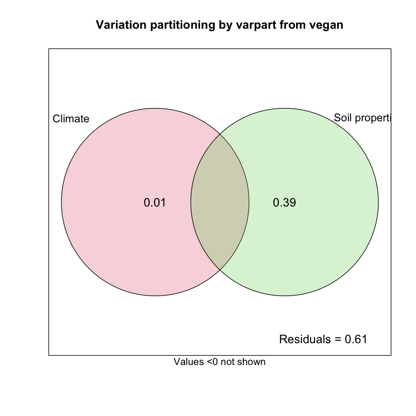
根据 RDA 和方差分解的结果(实际上是相同的结果),我们可以发现气候因素与土壤性质共同解释了 39.5% 的群落结构变异,其中土壤性质解释了 38.8% 的群落组成变异,气候解释了 0.2% 的群落组成变异。然而对于二者是否显著,还需要进一步检验。
# Define formula of soil property set and climate set to test.
# Set the variable from other category as condition
formula_soil <- formula(df_com ~ pH+MOI+TN+TP+NO3+SOC + Condition(MAT))
formula_clim <- formula(df_com ~ Condition(pH)+Condition(MOI)+Condition(TN)+Condition(TP)+Condition(NO3)+Condition(SOC) + MAT)

anova(rda(formula_soil, data = df_env))
## Permutation test for rda under reduced model
## Permutation: free
## Number of permutations: 999
##
## Model: rda(formula = df_com ~ pH + MOI + TN + TP + NO3 + SOC + Condition(MAT), data = df_env)
## Df Variance F Pr(>F)
## Model 6 842.8 17.025 0.001 ***
## Residual 142 1171.6
## ---
## Signif. codes: 0 '***' 0.001 '**' 0.01 '*' 0.05 '.' 0.1 ' ' 1anova(rda(formula_clim, data = df_env))## Permutation test for rda under reduced model
## Permutation: free
## Number of permutations: 999
##
## Model: rda(formula = df_com ~ Condition(pH) + Condition(MOI) + Condition(TN) + Condition(TP) + Condition(NO3) + Condition(SOC) + MAT, data = df_env)
## Df Variance F Pr(>F)
## Model 1 21.82 2.6443 0.071 .
## Residual 142 1171.56
## ---
## Signif. codes: 0 '***' 0.001 '**' 0.01 '*' 0.05 '.' 0.1 ' ' 1结合单因素方差分析 ANOVA 得到的结果,我们可以得出最终结论,土壤性质能够显著解释 38.8% 的群落组成变异,气候因素对于群落结构变异的解释不显著。