Han ([email protected]) 在最近刚刚完成的一篇 SCI 文章中,为了描述实验的采样范围,通过 ggplot2 包 (Wickham et al. 2019) 将一组 RasterLayer 绘制成为了青藏高原的地形图。考虑到使用 R 绘制地图的中文内容较少,我们进行一次回顾。
PS 因为不是地理方面的文章/专业,所以在专业性方面有欠缺,但对于自然科学类文章中进行展示基本上是足够了。
为什么用 ggplot2 画地图?
因为我能!(摊手
实际上原因如下:
-
ggplot2 是非常强大的绘图工具,配合上 ggplot2 的衍生包,这套工具链基本能满足生态学领域几乎所有的绘图需求。
-
如果对 Photoshop 这类图像处理软件熟悉,就会发现使用 ggplot2 画图,逻辑上和 PS 是非常相似的,便于快速上手和修改生成的图像——天知道把英文图改成中文图有多烦人
-
此外相比于 ArcGIS 这类软件 R 这类跨平台软件几乎可以在任何环境下完成绘图任务,甚至可以在家中的机顶盒安装 R,只不过慢到天长地久而已。
-
免费免费免费
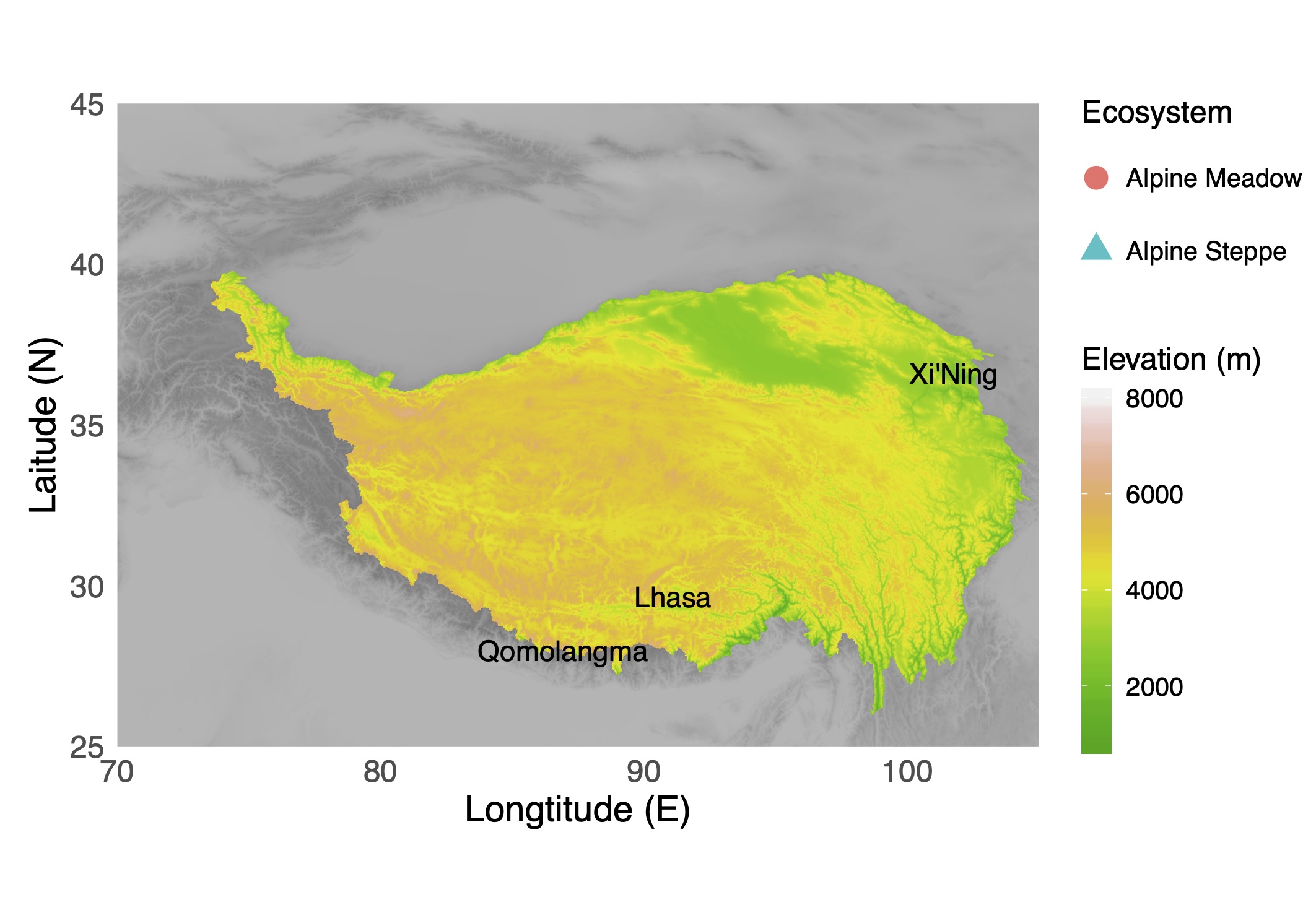
在开始之前,先来看看最终的展示效果。为了避免文章版权和数据共享问题,地图上样点均去除,仅供参考。
什么是 RasterLayer?
关于 RasterLayer 的定义,在 Spatial Data Science (Feed the Future n.d.) 中有很好的解释。
A RasterLayer object represents single-layer (variable) raster data. A RasterLayer object always stores a number of fundamental parameters that describe it. These include the number of columns and rows, the spatial extent, and the Coordinate Reference System. In addition, a RasterLayer can store information about the file in which the raster cell values are stored (if there is such a file). A RasterLayer can also hold the raster cell values in memory.
在 R 中提及的 RasterLayer 通常指的是由 sp 包 (Pebesma et al. 2019) 提供的 RasterLayer 类,每一个 RasterLayer 代表一层 raster 栅格数据,其中记录了 raster 数据的基础信息,例如行、列、空间范围、参考系。而对 RasterLayer 进行操作最常用的工具是 raster 包 (Hijmans et al. 2020)。
数据准备
所需加载包: 1. elevatr(Hollister and Shah 2018);2. raster; 3.tidyverse (Wickham and RStudio 2019)
具体到这一次的地图绘制中,我们需要两个 RasterLayer —— 1. 作为背景层的 bg_rst,以及 2.用作展示地形的 tp_rst。那么如何获得这两个 RasterLayer 呢?elevatr 包提供了专门用于获取高程栅格数据的方法 get_elev_raster.
不过在获取高程数据之前,需要首先指定地图绘制矩形边界。之后方可使用 get_elev_raster 来获取边界范围内的高程数据,使用 z 参数 (zoom) 确定缩放程度。因为通过 get_elev_raster 获取高程 raster 的方法是获取服务器与自定义边界的最小公倍数(不准确的说法),所以需要对获取的原始 RasterLayer 再次剪切,以便得到地图绘制矩形边界内的数据。
library(elevatr)  # Get rasterlay from AWS by `get_elev_raster` fucntion
library(raster)  # Manipulate RasterLayer object
library(tidyverse)  # Tidy is everything.

# Set the extent we want to plot
ext_sample <- extent(70, 105, 25, 45)

# Preparing for getting the elevation raster data, make a blank RasterLayer,
# becasue the first parameter of get_elev_raster is a target Rasterlayer.
bg_init <- raster(ext = ext_sample, resolution = 0.01)
# Get elevation raster with zoom 5, then only keep the extend we want to plot
# later.
bg_rst <- get_elev_raster(bg_init, z = 5) %>% crop(ext_sample)
bg_rst 就是地图背景中灰色的辅助部分的数据就准备好了。
# Let's check the detail of bg_rst, the Background RasterLayer
bg_rst
## class      : RasterLayer
## dimensions : 1075, 1591, 1710325  (nrow, ncol, ncell)
## resolution : 0.022, 0.0186  (x, y)
## extent     : 70.008, 105.01, 25.0029, 44.9979  (xmin, xmax, ymin, ymax)
## crs        : +proj=longlat +datum=WGS84 +ellps=WGS84 +towgs84=0,0,0
## source     : /private/var/folders/0s/pkk0623j6dgdq9yyg4d3qtq40000gn/T/RtmpUCKkKF/raster/r_tmp_2020-02-21_223346_8889_78742.grd
## names      : layer
## values     : -156.1392, 8006.811  (min, max)
随后我们需要下载青藏高原的多边形文件,这里我们选择张镱锂 (2002) 等人在《论青藏高原范围与面积》一文提供的青藏高原范围与界线地理信息系统数据。从《全球变化科学研究数据出版系统》下载即可。这里我选择了 DBATP.zip 下载,对应的文件格式为 Shaplefile,使用 rgdal 包 (Bivand et al. 2019) 提供的 readOGR 方法读取其中的 DBATP_Polygon.shp,保存的数据类型为tp_ext(类型为 SpatialPolygonsDataFrame)。之后将bg_rst 数据按照 tp_ext 形状进行处理,获得符合青藏高原范围的 RasterLayer tp_rst。
library(rgdal)
# Read the SpatialPolygon File from DBATP_Polygon.shp
tp_ext <- readOGR("DBATP/DBATP_Polygon.shp")
## OGR data source with driver: ESRI Shapefile
## Source: "/Users/chenhan/Documents/Develop Learn/R/plotMapByGGplot/DBATP/DBATP_Polygon.shp", layer: "DBATP_Polygon"
## with 1 features
## It has 1 fields
# Keep the shpae of the Tibetan Plateau
tp_rst <- mask(bg_rst, tp_ext)
为了便于定位,我们还将在图片上绘制地标名称 city_ls,以及采样点位置及其类型 hbt_coord。
PS.可以根据自己的实际情况确定数据的存储类型,这里因为个人项目的实际情况,数据并没有保存成为常见的 data.freame 或者 tibble 之类的类表格形式。注意绘图过程中前后对应即可。
# Create the list of landmarks which we want to mark
city_ls <- list(x = c(91.1, 86.925278, 101.7781), y = c(29.65, 27.988056, 36.6169),
    label = c("Lhasa", "Qomolangma", "Xi'Ning"))
str(city_ls)
## List of 3
##  $ x    : num [1:3] 91.1 86.9 101.8
##  $ y    : num [1:3] 29.6 28 36.6
##  $ label: chr [1:3] "Lhasa" "Qomolangma" "Xi'Ning"
# Read point with latitude and longitude. This operation is not needed for
# everyone, actually it depends on the actual data structure.
hbt_coord <- read_rds("hbt_coord.rds") %>% mutate(Ecosystem = ifelse(hbt == "M",
    "Alpine Meadow", "Alpine Steppe"))
str(hbt_coord)
## Classes 'tbl_df', 'tbl' and 'data.frame':    432 obs. of  4 variables:
##  $ hbt      : chr  "M" "M" "M" "M" ...
##  $ lon      : num  101 101 101 100 100 ...
##  $ lat      : num  35.3 35 35 34.5 34.5 ...
##  $ Ecosystem: chr  "Alpine Meadow" "Alpine Meadow" "Alpine Meadow" "Alpine Meadow" ...
注意,前面的操作中,我们裁剪 RasterLayer 用到了 crop 和 mask 两种操作,关于这两种操作的解释,我用一张图来解释:
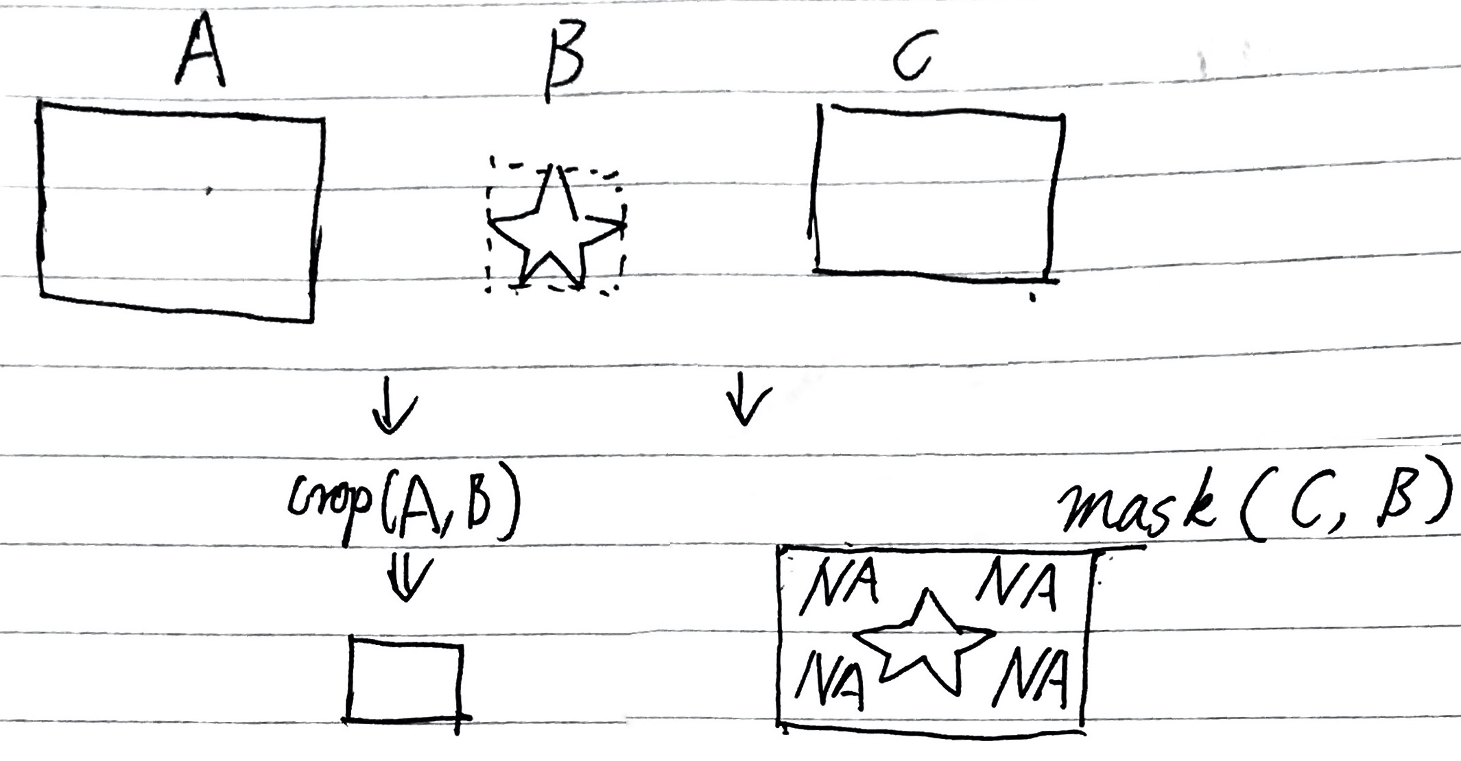
简而言之,两种操作都会得到更小的矩形图形,但是使用 mask 方法会在多边形区域外的矩形部分填充 NA 使被裁剪 RasterLayer 看起来成为多边形。
地图绘制
所需加载包: scales (Wickham, Seidel, and RStudio 2019)
不过在进行绘图之前,还需要对 RasterLayer 数据进行一些小的调整,以便与 ggplot2 的功能兼容。首先将两个 RasterLayer 转换为 data.frame 保留 xy,xy 为经纬度,应点上的值将会保留成与 RasterLayer 中 names 相同的列名,比如 bg_rst 转换为 data.frame 后列名就是 x, y, layer。之后我们将 layer(在此处为当前为止的海拔高度)转换数值范围,因为保留原始的数据用作后面的透明度会让整张图像灰蒙蒙。
不过要注意的是,正如我们前面说到的 mask 后的 RasterLayer 会将区域外的数据标记为 NA,如果直接使用 NA 绘图将会出现各种奇怪的效果,因此我们选择将 NA 数据更换为 0,将区域内的数据更换为 1,将两种值用作图像的 alpha 就会绘制出准确的青藏高原样式。
没看懂咋办?呆胶布!动手试试不进行 NA 转换的效果便知道了。
# scales package provide rescale function which can convert the range of numbers
# list to another range.
library(scales)
##
## Attaching package: 'scales'

## The following object is masked from 'package:purrr':
##
##     discard

## The following object is masked from 'package:readr':
##
##     col_factor
# First convert RasterLayer as Data.Frame with xy coordinate system.  Then
# rescale the elevaion to alpha, as the background part, super high alpha value
# is not a good idea, which range is the best? It depends by the actual. Save the
# alpha value with colname 'alpha'
bg_rst_df <- as.data.frame(bg_rst, xy = TRUE) %>% mutate(alpha = rescale(layer, to = c(0.25,
    0.75)))

# NA will be generated by the mask function, if use NA and evelation as the alpha
# of Topographic figure, it will be dizzy, and for color Topographic figure
# please don't use the greyscale and color for the evelation simultaneously. Just
# use alpha to control the shape of regional shpae.
tp_rst_df <- as.data.frame(tp_rst, xy = TRUE) %>% na.omit()
当数据准备完毕,我们就开始图形的绘制。首先进行地形图叠加到背景地形的绘制。因为命令较多,并且均以注释的形式标注到代码中,故此不再提前讲解。
# sacle_parm as a parameter controls the sclae of the hole figure, it will be
# used to control the size of text, point, legend, etc. to fit the size of
# figure.
scale_parm <- 2
# Init ggplot
# plot the backgroun layer, set the alpha without color will make a grey
# background
gmap <- ggplot() +
# plot the topographic layer, set alpha to keep the shape of Tibetan Plateau
# (TP). Color indicates the elevation.
geom_raster(data = bg_rst_df, aes(x = x, y = y, alpha = alpha)) +
 # terrain.colors is an built-in function to generate a list of color palettes.
# set the legend title of evelation by name parameter.
geom_raster(data = tp_rst_df, aes(x = x, y = y, fill = layer, alpha = alpha)) +
 # As we said before, the alphas is used to determine the shpae of TP, we don't
# need to show them as legends.
scale_fill_gradientn(colours = terrain.colors(100), name = "Elevation (m)") +
 # Project this figure as a map but not a normal figure
scale_alpha(guide = "none") +
 # Set preset theme makes things easire
coord_quickmap() +
 # Set the limititions of axes. `expand` parameter will remove the gaps between
theme_minimal() +
 # Set the titles of axis
scale_x_continuous(limits = c(70, 105), expand = c(0, 0)) + scale_y_continuous(limits = c(25,
    45), expand = c(0, 0)) +
labs(x = "Longtitude (E)", y = "Laitude (N)") +
 # remove the background color and background grid, you know the classical
# ggplot's grid, don't you?
theme(panel.grid = element_blank(), panel.background = element_blank()) +
# Set the size of axis and legend
theme(axis.title = element_text(size = 7 * scale_parm), axis.text = element_text(size = 6 *
    scale_parm)) + theme(legend.key.width = unit(0.2 * scale_parm, "cm"), legend.key.height = unit(0.5 *
    scale_parm, "cm"), legend.text = element_text(size = 5 * scale_parm), legend.title = element_text(size = 6 *
    scale_parm))

# Preview will slow down the process of operations, I highly recommand do not
# preveiw the ggplot and save it as a file directly.
上述操作完毕,如果没有意外,就可以获得一张效果尚可的底图了。但是,个人强烈建议不进行预览图像,直接进行后续的操作,因为绘制当前精度的底图需要花费较长的时间。或者可以使用 ggsave 方法输出为文件进行预览,这样如果效果满意,可以直接用作成品,避免预览后再次绘制效率较低。
随后我们再将地标为止添加到底图上。
gmap <- gmap +
  # Add the city_ls to the main plot as landmarks.
  geom_text(
    mapping = aes(x = x, y = y, label = label),
    # geom_text don't support the structure we used.
    # convert the list into data.frame, every element is used as column here.
    data = bind_cols(city_ls),
    size = 2 * scale_parm
  )
最后将采样点添加到底图上。注意 ⚠️ 由于版权和数据分享的原因,我将采样点的坐标设置为 0,0,故此图片上不会显示任何采样点,请根据实际情况设置!
gmap <- gmap +
  # Add the sample sites to the main plot as points.
  # Due to the copyright of my scholar article and data share policy, I won't point my sample sites to the picuture, the coordinations of point is 0,0 here.
  geom_point(
    mapping = aes(
      # x = lon,
      x = 0,
      y = 0,
      # y = lat,
      col = Ecosystem,
      shape = Ecosystem
    ),
    data = hbt_coord,
    # Don't set the size as 0 until you don't want to see anything here.
    # Don't set the size as 0 until you don't want to see anything here.
    # Don't set the size as 0 until you don't want to see anything here.
    size = 0 * scale_parm
  ) +
  # Convert the color as legend class, becasuse the shape legend is legend class.
  # If there is no class conversion, the shape and color will be showed as two legends.
  # Then select colour as guides and site a larger size to make it more readable.
  # Don't know what's these means? Commit below code will show you everything.
  scale_color_discrete(guide = "legend") +
  guides(colour = guide_legend(override.aes = list(size = .8 * scale_parm)))
如果对输出结果满意,那么可以跳过下面这一步,直接进行 ggsave 操作保存图像。不过在这里,保存图像之前,我们还需要修改图片的空白区域 margins 来让图像更合适一些。
gmap <- gmap +
  theme(plot.margin =
          # Set marigns of figure, the order of parameters is top, right, bottom, left
          unit(
            c(0 * scale_parm, 0 * scale_parm, -.2 * scale_parm, .2 * scale_parm),
            "cm"
          ))
最后导出图像即可。ggsvae 提供了丰富的参数定义输出的图像。对于需要投稿 SCI 的文章,通常 Author Guidelines 要求提供不低于 300 DPI 的图片文件。如果允许,保存为 PDF 文件会是不错的方法,毕竟通用性和文件大小都能得到很好的满足。
ggsave(filename = "gmap.pdf", plot = gmap, width = 9 * scale_parm, height = 6.2 *
    scale_parm, units = "cm", dpi = 600)
## Warning: Removed 432 rows containing missing values (geom_point).
最后,如果有任何更好的意见和建议,换用通过任何形式与我交流。祝大家都能制作出令自己(主要是杂志)满意的作品。
参考文献
Bivand, Roger, Tim Keitt, Barry Rowlingson, Edzer Pebesma, Michael Sumner, Robert Hijmans, Even Rouault, Frank Warmerdam, Jeroen Ooms, and Colin Rundel. 2019. “Rgdal: Bindings for the ’Geospatial’ Data Abstraction Library.” https://CRAN.R-project.org/package=rgdal.
Feed the Future. n.d. “Raster Data — R Spatial.” Blog. Spatial Data Science. Accessed February 19, 2020. https://rspatial.org/raster/spatial/4-rasterdata.html.
Hijmans, Robert J., Jacob van Etten, Michael Sumner, Joe Cheng, Andrew Bevan, Roger Bivand, Lorenzo Busetto, et al. 2020. “Raster: Geographic Data Analysis and Modeling.” https://CRAN.R-project.org/package=raster.
Hollister, Jeffrey, and Tarak Shah. 2018. “Elevatr: Access Elevation Data from Various APIs.” https://github.com/jhollist/elevatr.
Pebesma, Edzer, Roger Bivand, Barry Rowlingson, Virgilio Gomez-Rubio, Robert Hijmans, Michael Sumner, Don MacQueen, Jim Lemon, Josh O’Brien, and Joseph O’Rourke. 2019. “Sp: Classes and Methods for Spatial Data.” https://CRAN.R-project.org/package=sp.
Wickham, Hadley, Winston Chang, Lionel Henry, Thomas Lin Pedersen, Kohske Takahashi, Claus Wilke, Kara Woo, Hiroaki Yutani, and RStudio. 1. “Ggplot2: Create Elegant Data Visualisations Using the Grammar of Graphics.” https://CRAN.R-project.org/package=ggplot2.
Wickham, Hadley, and RStudio. 2019. “Tidyverse: Easily Install and Load the ’Tidyverse’.” https://CRAN.R-project.org/package=tidyverse.
Wickham, Hadley, Dana Seidel, and RStudio. 2019. “Scales: Scale Functions for Visualization.” https://CRAN.R-project.org/package=scales.
张镱锂, 李炳元, and 郑度. 2002. “论青藏高原范围与面积.” 地理学报 21 (1): 1–8. https://doi.org/10.11821/yj2002010001.